Spiral Positional-Encoding Benchmarks
real data · identical models · only the time features change
Does a transformer forecast better when time is supplied as temporalBLOCK spiral coordinates instead of a raw timestamp or plain calendar integers? We trained the same small transformer three times — same architecture, same data, same training budget — changing only the per-timestep time features. The spiral variant uses the exact encodeSpiral function that serves the production API.
The experiment
Task: predict New York City hourly temperature 24 hours ahead from the previous 96 hours. Data: 35,064 hours of Open-Meteo ERA5 reanalysis (2021–2024, UTC). Split: train on 2021–2023, test on all of 2024 — strictly chronological, no leakage. Model: 2-layer transformer (d_model 64, 4 heads), 4 epochs, best-validation checkpoint, 3 random seeds per variant.
| Variant | Time features per hour |
|---|---|
| A — raw | normalized unix-ms scalar (1 dim) |
| B — calendar | hour/24, weekday/7, month/12 (3 dims) |
| C — spiral | (sin θ, cos θ) × 12 scales from the production encoder (24 dims) |
Benchmark 1 — Forecast accuracy
Mean absolute error on unseen 2024 data, in °C (lower is better; mean of 3 seeds):
The spiral encoding cut forecast error by 22% vs. a raw timestamp and 16% vs. calendar integers, and won on every metric we tracked — including the boundary cases where integer features jump discontinuously while sin/cos stays smooth:
| Variant | MAE ± std | RMSE | Midnight ±1 h | Mondays |
|---|---|---|---|---|
| Raw unix timestamp | 4.18 ± 0.02 | 5.26 | 3.44 | 4.36 |
| Calendar integers | 3.87 ± 0.06 | 4.88 | 3.10 | 3.86 |
| temporalBLOCK spiral | 3.27 ± 0.14 | 4.18 | 2.97 | 3.55 |
Benchmark 2 — The advantage compounds with history
Same forecasting task as Benchmark 1 — NYC hourly temperature, 24 h ahead — but here we vary how much of the 2021–2023 training window is used (chronological tail, from ≈3.6 months up to the full three years; 2 seeds per point). The 36-month row uses the same training set as Benchmark 1, so its numbers are directly comparable (2 seeds here vs. 3 in Benchmark 1). At short history budgets the three encodings are statistically indistinguishable. The spiral variant separates clearly only when the full three years of pattern repetition are available:
| Training history | Raw | Calendar | Spiral* |
|---|---|---|---|
| ≈3.6 mo (2,616 h) | 4.56 | 4.29 | 4.33 |
| ≈9 mo (6,540 h) | 4.33 | 5.43 | 4.38 |
| ≈18 mo (13,080 h) | 4.25 | 4.04 | 4.03 |
| ≈36 mo (26,161 h) | 4.17 | 3.91 | 3.35 |
At the full three years, the spiral variant is 14% ahead of calendar features and 20% ahead of a raw timestamp. A plausible reading is that the richer 24-dimensional encoding needs enough repeated cycles (seasons, weeks, days) in the training data before the model can exploit it — consistent with, but not proven by, these four data points.
* all 12 scales, unfocused — the Spiral column above uses the full encoder without scale selection; each point is only 2 seeds, so small-data differences (including spiral's 3.6- and 9-month points and the calendar-integer 5.43 outlier at ≈9 months) are within noise. We report every measured number, so you can see where our strengths are.
Benchmark 3 — Selecting the band of scales
Scale selection is the encoding used well — the API exposes exactly this via a trusted-scales output, so a model consumes only the rungs its data needs. Hourly samples spanning three years call for the hour-through-year band (10 dims):
On the full training set (3 seeds: 2.92, 2.78, 2.73) the focus-band spiral reaches MAE 2.81 ± 0.08 °C — 14% below the all-scales spiral and 27% below calendar integers.
Note: focus-banding did not fix the small-data regime — at ≈3.6 months it was actually slightly worse than the full spiral (4.64 vs 4.33), at ≈18 months slightly better (3.86 vs 4.03). Its decisive win is at realistic data volumes.
Rule: keep a scale when its cycle length ≥ 2 × sample interval (Nyquist) and its full cycle fits at least once inside the training span.
Benchmark 4 — How many dimensions does accuracy cost?
Same task, full 36-month history, but sweeping nested bands of the spiral encoding from 2 dims (the daily rung alone) up to all 24 (3 seeds per band):
| Dims | Band | MAE ± std (°C) |
|---|---|---|
| 2 | hr | 3.97 ± 0.02 |
| 4 | hr–day | 2.85 ± 0.02 |
| 6 | hr–wk | 2.86 ± 0.08 |
| 8 | hr–mo | 2.87 ± 0.03 |
| 10 | hr–yr (auto-selected) | 2.81 ± 0.08 |
| 12 | min–yr | 3.07 ± 0.11 |
| 14 | s–yr | 2.76 ± 0.03 |
| 24 | us–mil (all scales) | 3.27 ± 0.14 |
Three things this table shows. First, 4 dimensions already capture almost the entire win — the hr + day rungs alone score 2.85, within noise of the best configurations. Second, adding sub-hour rungs (constant across hourly samples) is roughly harmless. Third, the real damage comes from the coarse rungs whose cycles the training window never completes — decade, century, millennium — which drag all-scales back to 3.27. Feature selection, not feature count, is what matters.
Note: the 10-dim hr–yr band (2.81 ± 0.08) is not hand-picked — it is exactly what the SDK's automatic scale selector (select_training_focus_band) returns for hourly samples over three years: keep a scale iff its cycle is ≥ 2× the sampling interval and completes within the training span. It is statistically level with the 14-dim s–yr band (2.76 ± 0.03) — we ship the auto-selected band rather than post-hoc picking the best row. The 12-dim min–yr point (3.07 ± 0.11) is noisier than its neighbours; we report it as measured.
Methodology
Public dataset, proprietary spiral encoder, 3 training scripts, no cherry-picking.
1. data     Open-Meteo ERA5 archive — NYC hourly temperature,
            2021-01-01 → 2024-12-31 UTC (35,064 hours)
2. encode   gen_spiral.mts — runs the production encodeSpiral()
            over every timestamp → 24-dim (sin, cos) features
3. train    train.py / train_efficiency.py / train_adaptive.py /
            train_dims_sweep.py — PyTorch, identical 2-layer
            transformer per variant, seeds 0-2, best-validation
            checkpoint → results.json
Benchmark 5 — Does temporal structure help an LLM in the prompt?
The first four benchmarks feed spiral coordinates to a model as numeric input features. This one asks a different question: if your events go to an LLM as text, does annotating each timestamp with its temporal structure improve the LLM's reasoning? 40 deterministic multiple-choice questions (same-time-of-day match, same-weekday match, broken 24 h cadence, exact-week-apart pair), each asked three ways to eight models from four vendors — six mid-tier plus two frontier models as a ceiling reference:
- ISO only — events with bare ISO-8601 UTC timestamps
- + spiral (sin, cos) — each event also carries raw spiral phase coordinates for the hr–yr band
- + Compact Spiral — the same phases as human-readable labels (
time-of-day:08:15UTC weekday:Fri week-of-year:wk11/52 …)
| Model | ISO only | + spiral (sin, cos) | + Compact Spiral |
|---|---|---|---|
| claude-sonnet-4-6 (Anthropic) | 83% | 90% | 85% |
| claude-opus-4-5 (Anthropic) | 65% | 57% | 80% |
| gpt-5.2 (OpenAI) | 75% | 80% | 100% |
| gpt-5.4 (OpenAI) | 78% | 78% | 98% |
| gemini-2.5-flash (Google) | 73% | 73% | 85% |
| deepseek-chat (DeepSeek) | 75% | 88% | 85% |
| claude-sonnet-5 (Anthropic) | 98% | 100% | 100% |
| gpt-5.6-terra (OpenAI) | 100% | 100% | 100% |
Every model here improves over bare ISO timestamps with at least one annotated format — but which format wins is model-dependent, not a universal rule. Three patterns across the six models:
- Compact Spiral wins for OpenAI: gpt-5.2 goes from 75% to 100% (30/40 → 40/40); gpt-5.4 from 78% to 98% (31/40 → 39/40). Spiral floats add nothing for either.
- Spiral floats win for DeepSeek: deepseek-chat goes from 75% to 88% (30/40 → 35/40). Compact Spiral is close behind (85%).
- Mixed for Anthropic: claude-sonnet-4-6 gains from both (+7pp spiral, +2pp compact). claude-opus-4-5 is hurt by raw floats (65% → 57%) but helped by Compact Spiral (26/40 → 32/40, +15pp) — different from claude-opus-5, which refused annotated prompts in both formats.
Does the gap widen on harder tasks?
We re-ran the four mid-tier models on a second, deliberately harder 40-question set: circular time-of-day distance across midnight, cumulative cadence drift over 20 events, a composite two-cycle (time-of-day AND weekday) match among 16 events, and a subtle <2 h anomaly hidden in 30 daily events. As a frontier reference on the same hard set, gpt-5.6-terra scores 100% in all three conditions and claude-sonnet-5 scores 95% ISO-only / 90% spiral / 95% compact — the hard set is where mid-tier formats separate:
| Model (hard set) | ISO only | + spiral (sin, cos) | + Compact Spiral |
|---|---|---|---|
| deepseek-chat (DeepSeek) | 78% | 100% | 88% |
| gpt-5.4 (OpenAI) | 43% | 68% | 48% |
| gemini-2.5-flash (Google) | 57% | 55% | 75% |
| claude-sonnet-4-6 (Anthropic) | 80% | 75% | 90% |
The spiral advantage widens where the model's favoured format already was spiral, and appears where it wasn't: deepseek-chat holds its +22pp spiral gain and reaches a perfect 40/40 while its ISO-only score stays flat, and gpt-5.4 — where spiral added nothing on the base set — gains +25pp from spiral floats on the hard set (17/40 → 27/40), overtaking its own compact-label format. For gemini-2.5-flash and claude-sonnet-4-6, Compact Spiral remains the better hard-set format (+18pp and +10pp over ISO-only respectively); raw floats do not help them. The model-dependence rule from the base set carries over — but on tasks that require genuinely circular reasoning, phase coordinates stop being redundant with what the model can derive itself.
Scope: one run per condition, 40 questions each, deterministic seeded question set — directional results on a narrow task, not a general model ranking. Frontier models are at the ceiling regardless of format — claude-sonnet-5 and gpt-5.6-terra in the table above score 98–100% across all three conditions, and gemini-2.5-pro, claude-opus-5, and gpt-5.5 score 100% from bare ISO timestamps — so the annotations matter for mid-tier models, not frontier ones. The likely reason: frontier models have deeply internalized Unix/ISO calendar conventions from training, so an alternative encoding adds prompt tokens without adding information they still need — and on longer prompts that extra weight can cost a point or two rather than help. That's why this benchmark targets the mid-tier, where the representation still changes the outcome. Small fast-tier models can get worse with raw coordinate floats (claude-haiku-4-5: 63% ISO-only → 50% with spiral floats). And One compatibility note: claude-opus-5 deterministically refused the annotated prompts in both formats (31/40 spiral, 40/40 compact) while answering the bare-ISO versions perfectly. Dense timestamp-annotation blocks can trip a model's internal safety classifier — not because the content is harmful, but because the structured coordinate syntax looks unfamiliar enough to trigger a cautious rejection. The API detects this automatically: when claude-opus-5 is the target model it strips the annotation block and sends the plain ISO timestamp instead, so the request goes through cleanly rather than returning a refusal. See the annotation guide for per-model format recommendations.
Benchmark 6 — What each annotation format costs in tokens
Prompt tokens are money and context budget. This measures the exact event-line renderings used in Benchmark 5, tokenized with o200k_base (the GPT-4o/5-family tokenizer) over 1,000 seeded events:
| Format | Tokens / event | vs plain ISO |
|---|---|---|
| Plain ISO timestamp | 19.0 | 1.00× |
| Hand-written prose date | 27.0 | 1.42× |
| Compact Spiral (terse) | 32.0 | 1.68× |
| Compact Spiral (verbose) | 48.0 | 2.53× |
| Spiral (sin, cos) floats (terse) | 49.0 | 2.58× |
| Spiral (sin, cos) floats (verbose) | 74.5 | 3.92× |
Read together with Benchmark 5, this settles which format to put in a prompt. The terse compact form — 18:36Z Thu wk8 Feb-2025 — carries the mid-tier accuracy gains at just 1.68× the tokens of a bare timestamp. All five Benchmark 5 mid-tier models were re-validated on both terse formats using the same 40-question set:
| Model | ISO only | terse spiral | terse compact |
|---|---|---|---|
| deepseek-chat (DeepSeek) | 70% | 85% | 70% |
| gpt-5.2 (OpenAI) | 80% | 83% | 95% |
| claude-sonnet-4-6 (Anthropic) | 75% | 78% | 83% |
| gpt-5.4 (OpenAI) | 75% | 73% | 98% |
| gemini-2.5-flash (Google) | 78% | 70% | 80% |
Terse compact matched or beat plain on every model; terse spiral kept DeepSeek's advantage (85% vs 70%). In absolute terms the overhead is small: terse compact adds 13 tokens per event — roughly 13k tokens per 1,000 annotated events, which is well under a cent at typical input-token pricing. The multiplier only matters at extreme scale or when pressed against a context window. The (sin, cos) coordinates earn their keep where nothing else works: as numeric features for trained models (Benchmarks 1–4) and as distance metrics for retrieval (Benchmark 8, below) — not as prompt text.
Benchmark 7 — Do annotations reduce temporal hallucination?
The previous benchmarks measure whether temporal context helps a model answer correctly. This one asks the opposite: does it help a model refuse to answer when a question is unanswerable? 40 MCQ questions with an explicit abstain option (“None of the above / cannot be determined”): 20 traps across four categories — events matching no listed option, phantom event labels, questions that hinge on an unspecified local timezone, and false premises baked into the question — plus 20 matched answerable controls. The metric is fabrication rate: how often a model commits to an answer on a trap instead of abstaining.
The intervention is the product's recommended integration: a real POST /v1/calibrate calibrationBlock prefixed to the prompt, plus a one-sentence guard clause stating what the calibration does not reveal (local timezones, premise validity). With the block in place, sonnet-4-6, o4-mini, and gemini-2.5-flash all drop to 0% fabrication, while gpt-5.4-mini and deepseek-chat hold steady or improve.
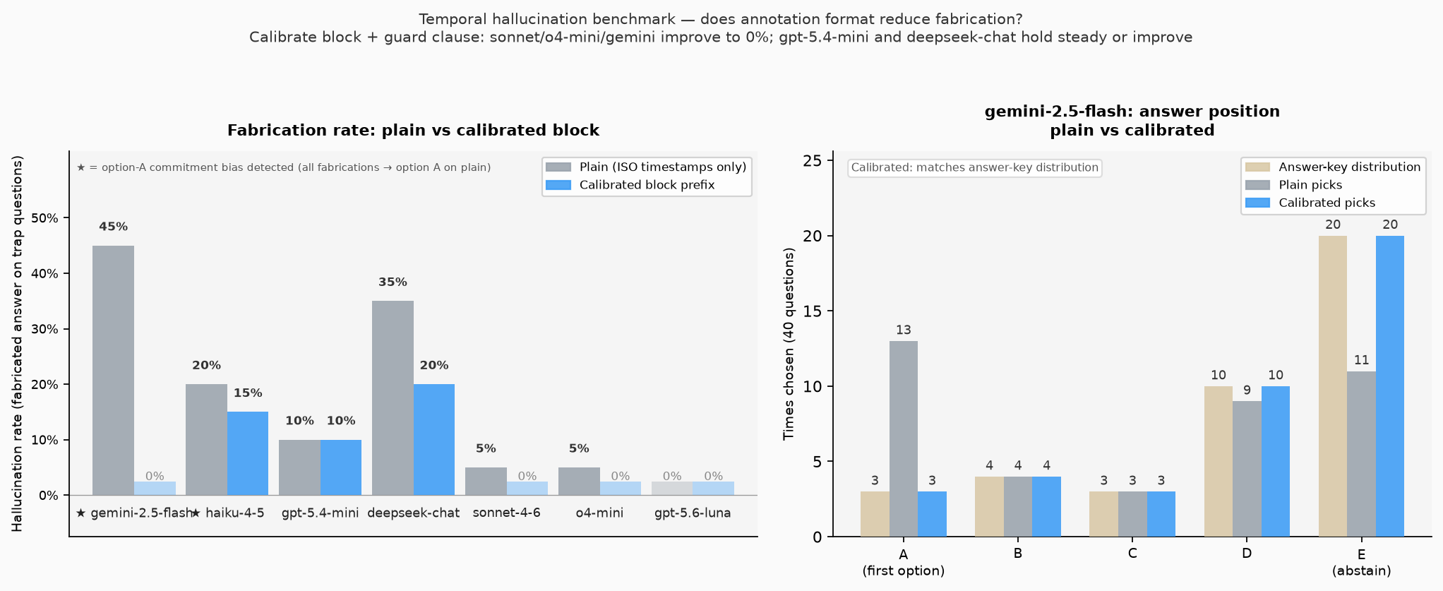
The standout is gemini-2.5-flash, and the right panel shows why. Under plain ISO timestamps, every one of its nine fabrications picked option A — the first-listed plausible distractor — and it abstained zero times where it should have abstained twenty. That's not diffuse confusion; it's a specific first-option commitment bias on unanswerable questions. With the calibration block prefixed, its answer distribution matches the answer key exactly: 45% fabrication → 0%, 40 of 40 correct, from a prefix that adds no per-event annotations at all.
Benchmark 8 — Retrieval: finding events at similar times
Vector search and RAG pipelines retrieve by nearest-neighbor distance. If your query is "events at a similar time" — same time of day, same point in the week or year — the timestamp representation is the distance metric. This benchmark is model-free: 5,000 seeded events over two years, brute-force kNN under three representations, scored by R-precision (retrieve exactly as many items as are truly relevant; report the fraction that are). Queries are half uniform, half near a cycle boundary — midnight or year-end — where wrap-around bites:
| Task | Representation | Overall | At boundary |
|---|---|---|---|
| Time of day (±15 min) | Unix timestamp | 0.021 | 0.021 |
| Time of day (±15 min) | Calendar integers | 0.899 | 0.804 |
| Time of day (±15 min) | Spiral (sin, cos) | 1.000 | 1.000 |
| Weekday + time of day | Unix timestamp | 0.011 | 0.010 |
| Weekday + time of day | Calendar integers | 0.825 | 0.663 |
| Weekday + time of day | Spiral (sin, cos) | 0.806 | 0.626 |
| Annual phase (±10 days) | Unix timestamp | 0.473 | 0.445 |
| Annual phase (±10 days) | Calendar integers | 0.878 | 0.777 |
| Annual phase (±10 days) | Spiral (sin, cos) | 0.994 | 1.000 |
The structural point: a linear representation cannot wrap. For a query at 23:58, roughly half its true time-of-day neighbors sit just past midnight — at the far end of a linear scale, where plain Euclidean nearest-neighbor search can never reach them (you'd have to add a wrap-aware distance function or a learned transform on top). Spiral coordinates place 23:58 and 00:06 next to each other by construction: 1.000 vs 0.804 at the midnight boundary on time-of-day retrieval, and 1.000 vs 0.777 at the year boundary for annual-phase retrieval. Raw Unix timestamps fail the task entirely (0.021 overall) — temporal adjacency and temporal phase similarity are different questions.
Note: on the composite weekday + time-of-day task, calendar and spiral representations score in the same range (0.825 vs 0.806 overall) — the ground truth treats weekday as discrete, which neither continuous encoding matches exactly. The spiral advantage shown here is on single-cycle phase tasks (time of day, annual phase) at their wrap boundaries.
Benchmark 9 — Long context: 300-event haystacks
Do the annotation gains survive when the event list grows from a few dozen lines to 300? Same question types as Benchmark 5, but each prompt carries a 300-event haystack (20 questions per condition, deterministic seeds).
| Model | Plain ISO | + Spiral floats | + Compact Spiral |
|---|---|---|---|
| gpt-5.6-terra(frontier) | 100% | 100% | 100% |
| claude-sonnet-4-6(mid) | 85% | 65% | 90% |
| gpt-5.2(mid) | 85% | 80% | 90% |
| deepseek-chat(mid) | 80% | 75% | 90% |
| gemini-3-flash-preview(lite) | 90% | 95% | 80% |
| claude-haiku-4-5(lite) | 60% | 65% | 45% |
Three patterns emerge across the six models. Frontier: gpt-5.6-terra hits 100% in every condition. Mid-tier: claude-sonnet-4-6 plain 85% rises to Compact 90% but drops to 65% with Spiral floats — extra tokens per line add noise once the context is already rich. gpt-5.2 and deepseek-chat both peak at 90% Compact, consistent with the short-prompt result. Lite: gemini-3-flash-preview is the standout — 95% Spiral, the highest annotated score in the table and the only lite model that benefits from full float annotations at scale. claude-haiku-4-5 goes the other direction: 60% plain, 65% Spiral, then collapses to 45% Compact — annotations actively hurt it at 300-event depth.
Benchmark 10 — Does fine-tuning on spiral-annotated data improve temporal reasoning?
Benchmarks 5–9 show annotation helps mid-tier models at inference time. This asks a different question: if you fine-tune a small model specifically on spiral- or compact-annotated training data, does it reason about time better than a model fine-tuned on the same questions with plain ISO timestamps?
Base model: Qwen2.5-3B-Instruct. Three LoRA adapters (r=16, α=32, 2 epochs) trained on 1,500 chat examples each — one per annotation format — then evaluated on the exact 40-question set from Benchmark 5. ft-plain is the control: the annotation format can only claim credit if ft-spiral or ft-compact beats it.
| Arm | Correct | Accuracy | vs control |
|---|---|---|---|
| base / plain | 17 / 40 | 42% | — |
| base / spiral | 13 / 40 | 32% | −10pp (annotation hurts untrained model) |
| base / compact | 16 / 40 | 40% | −2pp |
| ft-plain / plain | 34 / 40 | 85% | control (+43pp over base) |
| ft-spiral / spiral | 33 / 40 | 82% | −2pp vs control (within noise) |
| ft-compact / compact | 33 / 40 | 82% | −2pp vs control (within noise) |
Fine-tuning works: a 3B model jumps from 42% to 85% on this question set after seeing 1,500 annotated examples — a +43 percentage-point gain. The annotation format does not add further lift once the model has been fine-tuned (ft-spiral and ft-compact land within 2pp of ft-plain, well inside single-run noise for 40 questions). Note that annotation format is a prompt-time lever for models you can't retrain; for models you can fine-tune, the training signal matters far more than the format. The base-model rows also confirm Benchmark 5's finding from the other direction — an un-fine-tuned small model gets slightly worse when you add spiral floats (32% vs 42% plain), because it has no learned prior for the coordinate syntax.
Replication on a second architecture: Llama-3.2-3B-Instruct
Same kit, second base model, and this time the full cross-evaluation grid: every adapter evaluated under every prompt format, not just its own. Rows are what the adapter was trained on; columns are what it was prompted with at eval time.
| Adapter ↓ / Prompt → | plain | spiral | compact |
|---|---|---|---|
| base (no adapter) | 2 / 40 | 1 / 40 | 4 / 40 |
| ft-plain | 25 / 40 | 24 / 40 | 25 / 40 |
| ft-spiral | 13 / 40 | 17 / 40 | 18 / 40 |
| ft-compact | 18 / 40 | 17 / 40 | 26 / 40 |
Again, here we see the base model is near floor (5% plain) — the eval set punishes an untrained 3B model hard. Fine-tuning on plain data lifts it to 62% and generalizes across all three prompt formats (24–25/40 everywhere): the plain-trained model learned temporal reasoning, not a format. The spiral-trained adapter learned the format instead: it drops to 13/40 when prompted without its coordinates and never recovers the control's level even with them (17/40). ft-compact/compact posts the single best cell (26/40, 65%) — one question above the control, within single-run noise — while also degrading less off-format than ft-spiral. Two architectures now agree: the training signal dominates, compact annotations are format-robust, while raw spiral floats can make a small model brittle.
Benchmark 10.5 — What if the model learns to read spiral coords instead?
All three fine-tune runs trained the model to output spiral coordinates. The natural next step inverts the direction: train the model to consume spiral coordinates as input context, with no ISO timestamp to fall back on. The first grounding adapter (1,500 examples, 2 epochs, QLoRA 4-bit, ~12 min) more than tripled the base model's delta score — confirming the model learned to decode coordinates rather than ignore them. A v2 run with decode-trace CoT, 6,000 examples, and a larger adapter (r=32 + MLP projections) shows significant improvement over the base LoRA baseline.
| Model | with-spiral | without-spiral | delta |
|---|---|---|---|
| base (no adapter) | 12 / 40 | 7 / 40 | +5 |
| ft-grounding v1 | 21 / 40 | 4 / 40 | +17 |
| ft-grounding v2 | 40 / 40 | 0 / 40 | +40 |
| ft-grounding v2 · MathCoder2 base | 40 / 40 | 14 / 40 | +26 |
The v2 result replicated on a second base model (MathCoder2-Llama-3-8B): 40/40 with coordinates, and — unlike the first run — the without-coordinates arm held at the base model's own 14/40 instead of collapsing, so the entire +26 delta is attributable to reading the coordinates. See the development log for the full replication details.
Grounding development log →
Full experiment detail: v1 results, v2 design rationale, and training curves
Benchmark 11 — Cyclic turbulence: when time wraps around
Benchmarks 5–9 mostly test pattern-matching on clean timestamp lists. This set is built to be cyclically nasty: 60 deterministic questions where the right answer requires treating time as a set of cycles, seeded with the calendar's worst edge cases — midnight wrap-around (23:50 vs 00:15 are 25 minutes apart, not 23½ hours), Dec/Jan month-phase traps, a leap-day distractor, year-boundary dates that belong to the previous ISO year, and the 53-week ISO year 2026.
Six question types: same quarter across years, circular time-of-day proximity, exact 12-hour antiphase, month-of-year matching, weekday + day-segment harmonic alignment, and ISO week numbers. Same three conditions as Benchmark 5: plain ISO timestamps, spiral coordinates, and compact human-readable phase labels.
| Model | Plain | Spiral | Compact | Best lift |
|---|---|---|---|---|
| deepseek-chat | 58% | 93% | 78% | +35pp (spiral) |
| gpt-5.2 | 33% | 50% | 72% | +39pp (compact) |
| gemini-2.5-flash | 58% | 53% | 88% | +30pp (compact) |
| claude-haiku-4-5 | 68% | 58% | 73% | +5pp (compact) |
| claude-sonnet-4-6 | 93% | 82% | 100% | +7pp (compact) |
| gemini-2.5-pro | 100% | 90% | 100% | at ceiling on plain |
| gpt-5.6-luna | 98% | 100% | 93% | at ceiling |
| claude-sonnet-5 | 100% | 97% | 100% | at ceiling on plain |
The pattern from Benchmark 5 holds and sharpens. For mid-tier models, annotation is the difference between failing and passing: gpt-5.2 more than doubles from 33% to 72% with Compact Spiral (+39pp, the largest single-condition lift we've measured on any set), and deepseek-chat jumps from 58% to 93% with spiral coordinates (35/60 → 56/60). Frontier models (gemini-2.5-pro, gpt-5.6-luna) solve the cyclic turbulence from raw ISO strings alone and have nothing left to gain. And the model-dependence is real: both Anthropic models score lower with spiral floats than plain here, which is exactly why the API's adaptive annotation selector picks the format per model instead of always sending spiral.
What the data says
Across benchmarks 5–11, a few patterns hold consistently.
Frontier models (gpt-5.6-terra, gemini-2.5-pro, sonnet 5) approach ceiling on most simpler calendar-question sets regardless of format, so annotation adds little measurable lift here — but also causes no regression, meaning these models can use the API safely without custom tuning. Future benchmarks are being designed to push these newer models further.
Mid-tier models show the most consistent gains overall: lifts across all sets come from this group and the pattern continues with more difficult runs. These models are powerful enough to recognize and benefit from the connection without losing focus.
Lite models are the most format-sensitive and are more likely to degrade without fine-tuning. Model-specific adjustments will be maintained.
A major takeaway from these benchmarks is that ISO-only integration is already deeply embedded in systems training, yet does not appear to be the most effective approach to time mapping — simple and complex systems improve with spiral calibrations, while ISO accuracy only holds up when backed by expensive high-end processing. Lower-tier models were able to meet a higher standard with minor calibrations, and those trained exclusively on spiral strings showed the largest gains.
Cheap data requires a stronger system to extract gains; but a data-rich spiral system delivers higher accuracy natively, with the largest potential insights expected in high-tier models trained directly on it. New data to follow.
temporalBLOCK benchmark team